Quick Start: Tilt Series
In this guide, you will learn how to process your tilt series data all the way from frames and associated metadata to a nice high resolution map from the command line using WarpTools! 🌟
We will be processing 5 tilt series of apoferritin from EMPIAR-10491 as an example in this guide.
You should obtain a ~3Å map from these 5 tilt series following this guide.

Overview
- frame series preprocessing with WarpTools
- tilt series preprocessing with WarpTools
- initial 3D refinement in RELION
- multi-particle refinement with MTools and MCore
Pre-Calculated Results
Pre-calculated results (38GB) are available to download at 10.5281/zenodo.11398168.
Preparation
Download the data
First, let's download the frame series data, mdoc metadata files and the gain reference into an empty directory.
only have tilt series stacks?
Check our guide on processing tilt series stacks to get started!
# download the gain reference
wget \
--timestamping \
--no-directories \
--directory-prefix ./ \
ftp://ftp.ebi.ac.uk/empiar/world_availability/10491/data/gain_ref.mrc;

for i in 1 11 17 23 32;
do
    echo "======================================================"
    echo "================= Downloading TS_${i} ================"
    # download the mdoc file
    wget \
    --timestamping \
    --no-directories \
    --directory-prefix ./mdoc \
    ftp://ftp.ebi.ac.uk/empiar/world_availability/10491/data/tiltseries/mdoc/TS_${i}.mrc.mdoc;

    # download the frames
    wget \
    --timestamping \
    --no-directories \
    --directory-prefix ./frames \
    ftp://ftp.ebi.ac.uk/empiar/world_availability/10491/data/tiltseries/data/*-${i}_*.tif;
done
.
├── gain_ref.mrc
├── frames
└── mdoc

2 directories, 1 file
./frames
├── 2Dvs3D_53-1_00001_-0.0_Jul31_10.36.03.tif
├── 2Dvs3D_53-1_00002_2.0_Jul31_10.36.43.tif
├── 2Dvs3D_53-1_00003_4.0_Jul31_10.37.23.tif
├── 2Dvs3D_53-1_00004_-2.0_Jul31_10.38.06.tif
├── 2Dvs3D_53-1_00005_-4.0_Jul31_10.38.47.tif
├── 2Dvs3D_53-1_00006_6.0_Jul31_10.39.28.tif
├── 2Dvs3D_53-1_00007_8.0_Jul31_10.40.08.tif
├── 2Dvs3D_53-1_00008_-6.0_Jul31_10.40.51.tif
├── 2Dvs3D_53-1_00009_-8.0_Jul31_10.41.34.tif
├── 2Dvs3D_53-1_00010_10.0_Jul31_10.42.16.tif
├── 2Dvs3D_53-1_00011_12.0_Jul31_10.42.56.tif
├── 2Dvs3D_53-1_00012_-10.0_Jul31_10.43.39.tif
├── 2Dvs3D_53-1_00013_-12.0_Jul31_10.44.21.tif
├── 2Dvs3D_53-1_00014_14.0_Jul31_10.45.03.tif
├── 2Dvs3D_53-1_00015_16.0_Jul31_10.45.51.tif
├── 2Dvs3D_53-1_00016_-14.0_Jul31_10.46.47.tif
├── 2Dvs3D_53-1_00017_-16.0_Jul31_10.47.29.tif
├── 2Dvs3D_53-1_00018_18.0_Jul31_10.48.13.tif
├── 2Dvs3D_53-1_00019_20.0_Jul31_10.48.53.tif
├── 2Dvs3D_53-1_00020_-18.0_Jul31_10.49.38.tif
├── 2Dvs3D_53-1_00021_-20.0_Jul31_10.50.20.tif
├── 2Dvs3D_53-1_00022_22.0_Jul31_10.51.04.tif
├── 2Dvs3D_53-1_00023_24.0_Jul31_10.51.44.tif
├── 2Dvs3D_53-1_00024_-22.0_Jul31_10.52.29.tif
├── 2Dvs3D_53-1_00025_-24.0_Jul31_10.53.10.tif
├── 2Dvs3D_53-1_00026_26.0_Jul31_10.53.54.tif
├── 2Dvs3D_53-1_00027_28.0_Jul31_10.54.34.tif
├── 2Dvs3D_53-1_00028_-26.0_Jul31_10.55.20.tif
├── 2Dvs3D_53-1_00029_-28.0_Jul31_10.56.01.tif
├── 2Dvs3D_53-1_00030_30.0_Jul31_10.56.46.tif
├── 2Dvs3D_53-1_00031_32.0_Jul31_10.57.26.tif
├── 2Dvs3D_53-1_00032_-30.0_Jul31_10.58.12.tif
├── 2Dvs3D_53-1_00033_-32.0_Jul31_10.59.02.tif
├── 2Dvs3D_53-1_00034_34.0_Jul31_10.59.47.tif
├── 2Dvs3D_53-1_00035_36.0_Jul31_11.00.36.tif
├── 2Dvs3D_53-1_00036_-34.0_Jul31_11.01.23.tif
├── 2Dvs3D_53-1_00037_-36.0_Jul31_11.02.04.tif
├── 2Dvs3D_53-1_00038_38.0_Jul31_11.03.02.tif
├── 2Dvs3D_53-1_00039_40.0_Jul31_11.03.42.tif
├── 2Dvs3D_53-1_00040_-38.0_Jul31_11.04.30.tif
├── 2Dvs3D_53-1_00041_-40.0_Jul31_11.05.12.tif
├── 2Dvs3D_53-11_00001_-0.0_Jul31_16.50.54.tif
├── 2Dvs3D_53-11_00002_2.0_Jul31_16.51.34.tif
├── 2Dvs3D_53-11_00003_4.0_Jul31_16.52.14.tif
├── 2Dvs3D_53-11_00004_-2.0_Jul31_16.52.57.tif
├── 2Dvs3D_53-11_00005_-4.0_Jul31_16.53.38.tif
├── 2Dvs3D_53-11_00006_6.0_Jul31_16.54.20.tif
├── 2Dvs3D_53-11_00007_8.0_Jul31_16.54.59.tif
├── 2Dvs3D_53-11_00008_-6.0_Jul31_16.55.43.tif
├── 2Dvs3D_53-11_00009_-8.0_Jul31_16.56.25.tif
├── 2Dvs3D_53-11_00010_10.0_Jul31_16.57.07.tif
├── 2Dvs3D_53-11_00011_12.0_Jul31_16.57.47.tif
├── 2Dvs3D_53-11_00012_-10.0_Jul31_16.58.31.tif
├── 2Dvs3D_53-11_00013_-12.0_Jul31_16.59.13.tif
├── 2Dvs3D_53-11_00014_14.0_Jul31_16.59.55.tif
├── 2Dvs3D_53-11_00015_16.0_Jul31_17.00.35.tif
├── 2Dvs3D_53-11_00016_-14.0_Jul31_17.01.19.tif
├── 2Dvs3D_53-11_00017_-16.0_Jul31_17.02.01.tif
├── 2Dvs3D_53-11_00018_18.0_Jul31_17.02.52.tif
├── 2Dvs3D_53-11_00019_20.0_Jul31_17.03.33.tif
├── 2Dvs3D_53-11_00020_-18.0_Jul31_17.04.18.tif
├── 2Dvs3D_53-11_00021_-20.0_Jul31_17.05.08.tif
├── 2Dvs3D_53-11_00022_22.0_Jul31_17.05.52.tif
├── 2Dvs3D_53-11_00023_24.0_Jul31_17.06.32.tif
├── 2Dvs3D_53-11_00024_-22.0_Jul31_17.07.18.tif
├── 2Dvs3D_53-11_00025_-24.0_Jul31_17.07.59.tif
├── 2Dvs3D_53-11_00026_26.0_Jul31_17.08.44.tif
├── 2Dvs3D_53-11_00027_28.0_Jul31_17.09.24.tif
├── 2Dvs3D_53-11_00028_-26.0_Jul31_17.10.09.tif
├── 2Dvs3D_53-11_00029_-28.0_Jul31_17.10.51.tif
├── 2Dvs3D_53-11_00030_30.0_Jul31_17.11.37.tif
├── 2Dvs3D_53-11_00031_32.0_Jul31_17.12.17.tif
├── 2Dvs3D_53-11_00032_-30.0_Jul31_17.13.23.tif
├── 2Dvs3D_53-11_00033_-32.0_Jul31_17.14.05.tif
├── 2Dvs3D_53-11_00034_34.0_Jul31_17.14.51.tif
├── 2Dvs3D_53-11_00035_36.0_Jul31_17.15.31.tif
├── 2Dvs3D_53-11_00036_-34.0_Jul31_17.16.18.tif
├── 2Dvs3D_53-11_00037_-36.0_Jul31_17.17.00.tif
├── 2Dvs3D_53-11_00038_38.0_Jul31_17.17.46.tif
├── 2Dvs3D_53-11_00039_40.0_Jul31_17.18.26.tif
├── 2Dvs3D_53-11_00040_-38.0_Jul31_17.19.13.tif
├── 2Dvs3D_53-11_00041_-40.0_Jul31_17.19.55.tif
├── 2Dvs3D_53-17_00001_-0.0_Jul31_21.21.04.tif
├── 2Dvs3D_53-17_00002_2.0_Jul31_21.21.44.tif
├── 2Dvs3D_53-17_00003_4.0_Jul31_21.22.24.tif
├── 2Dvs3D_53-17_00004_-2.0_Jul31_21.23.07.tif
├── 2Dvs3D_53-17_00005_-4.0_Jul31_21.23.48.tif
├── 2Dvs3D_53-17_00006_6.0_Jul31_21.24.29.tif
├── 2Dvs3D_53-17_00007_8.0_Jul31_21.25.09.tif
├── 2Dvs3D_53-17_00008_-6.0_Jul31_21.25.53.tif
├── 2Dvs3D_53-17_00009_-8.0_Jul31_21.26.34.tif
├── 2Dvs3D_53-17_00010_10.0_Jul31_21.27.17.tif
├── 2Dvs3D_53-17_00011_12.0_Jul31_21.27.56.tif
├── 2Dvs3D_53-17_00012_-10.0_Jul31_21.28.41.tif
├── 2Dvs3D_53-17_00013_-12.0_Jul31_21.29.23.tif
├── 2Dvs3D_53-17_00014_14.0_Jul31_21.30.07.tif
├── 2Dvs3D_53-17_00015_16.0_Jul31_21.30.47.tif
├── 2Dvs3D_53-17_00016_-14.0_Jul31_21.31.43.tif
├── 2Dvs3D_53-17_00017_-16.0_Jul31_21.32.25.tif
├── 2Dvs3D_53-17_00018_18.0_Jul31_21.33.08.tif
├── 2Dvs3D_53-17_00019_20.0_Jul31_21.33.47.tif
├── 2Dvs3D_53-17_00020_-18.0_Jul31_21.34.32.tif
├── 2Dvs3D_53-17_00021_-20.0_Jul31_21.35.14.tif
├── 2Dvs3D_53-17_00022_22.0_Jul31_21.35.58.tif
├── 2Dvs3D_53-17_00023_24.0_Jul31_21.36.38.tif
├── 2Dvs3D_53-17_00024_-22.0_Jul31_21.37.24.tif
├── 2Dvs3D_53-17_00025_-24.0_Jul31_21.38.07.tif
├── 2Dvs3D_53-17_00026_26.0_Jul31_21.38.51.tif
├── 2Dvs3D_53-17_00027_28.0_Jul31_21.39.31.tif
├── 2Dvs3D_53-17_00028_-26.0_Jul31_21.40.17.tif
├── 2Dvs3D_53-17_00029_-28.0_Jul31_21.41.07.tif
├── 2Dvs3D_53-17_00030_30.0_Jul31_21.41.51.tif
├── 2Dvs3D_53-17_00031_32.0_Jul31_21.42.31.tif
├── 2Dvs3D_53-17_00032_-30.0_Jul31_21.43.18.tif
├── 2Dvs3D_53-17_00033_-32.0_Jul31_21.44.01.tif
├── 2Dvs3D_53-17_00034_34.0_Jul31_21.44.45.tif
├── 2Dvs3D_53-17_00035_36.0_Jul31_21.45.26.tif
├── 2Dvs3D_53-17_00036_-34.0_Jul31_21.46.12.tif
├── 2Dvs3D_53-17_00037_-36.0_Jul31_21.46.55.tif
├── 2Dvs3D_53-17_00038_38.0_Jul31_21.47.40.tif
├── 2Dvs3D_53-17_00039_40.0_Jul31_21.48.20.tif
├── 2Dvs3D_53-17_00040_-38.0_Jul31_21.49.08.tif
├── 2Dvs3D_53-17_00041_-40.0_Jul31_21.49.50.tif
├── 2Dvs3D_53-23_00001_-0.0_Aug01_10.29.18.tif
├── 2Dvs3D_53-23_00002_2.0_Aug01_10.29.58.tif
├── 2Dvs3D_53-23_00003_4.0_Aug01_10.30.39.tif
├── 2Dvs3D_53-23_00004_-2.0_Aug01_10.31.21.tif
├── 2Dvs3D_53-23_00005_-4.0_Aug01_10.32.02.tif
├── 2Dvs3D_53-23_00006_6.0_Aug01_10.32.43.tif
├── 2Dvs3D_53-23_00007_8.0_Aug01_10.33.23.tif
├── 2Dvs3D_53-23_00008_-6.0_Aug01_10.34.06.tif
├── 2Dvs3D_53-23_00009_-8.0_Aug01_10.34.48.tif
├── 2Dvs3D_53-23_00010_10.0_Aug01_10.35.30.tif
├── 2Dvs3D_53-23_00011_12.0_Aug01_10.36.10.tif
├── 2Dvs3D_53-23_00012_-10.0_Aug01_10.36.53.tif
├── 2Dvs3D_53-23_00013_-12.0_Aug01_10.37.34.tif
├── 2Dvs3D_53-23_00014_14.0_Aug01_10.38.17.tif
├── 2Dvs3D_53-23_00015_16.0_Aug01_10.38.58.tif
├── 2Dvs3D_53-23_00016_-14.0_Aug01_10.39.42.tif
├── 2Dvs3D_53-23_00017_-16.0_Aug01_10.40.24.tif
├── 2Dvs3D_53-23_00018_18.0_Aug01_10.41.07.tif
├── 2Dvs3D_53-23_00019_20.0_Aug01_10.41.47.tif
├── 2Dvs3D_53-23_00020_-18.0_Aug01_10.42.32.tif
├── 2Dvs3D_53-23_00021_-20.0_Aug01_10.43.14.tif
├── 2Dvs3D_53-23_00022_22.0_Aug01_10.43.57.tif
├── 2Dvs3D_53-23_00023_24.0_Aug01_10.44.38.tif
├── 2Dvs3D_53-23_00024_-22.0_Aug01_10.45.24.tif
├── 2Dvs3D_53-23_00025_-24.0_Aug01_10.46.06.tif
├── 2Dvs3D_53-23_00026_26.0_Aug01_10.46.50.tif
├── 2Dvs3D_53-23_00027_28.0_Aug01_10.47.31.tif
├── 2Dvs3D_53-23_00028_-26.0_Aug01_10.48.16.tif
├── 2Dvs3D_53-23_00029_-28.0_Aug01_10.48.58.tif
├── 2Dvs3D_53-23_00030_30.0_Aug01_10.49.50.tif
├── 2Dvs3D_53-23_00031_32.0_Aug01_10.50.30.tif
├── 2Dvs3D_53-23_00032_-30.0_Aug01_10.51.17.tif
├── 2Dvs3D_53-23_00033_-32.0_Aug01_10.51.59.tif
├── 2Dvs3D_53-23_00034_34.0_Aug01_10.52.51.tif
├── 2Dvs3D_53-23_00035_36.0_Aug01_10.53.39.tif
├── 2Dvs3D_53-23_00036_-34.0_Aug01_10.54.28.tif
├── 2Dvs3D_53-23_00037_-36.0_Aug01_10.55.10.tif
├── 2Dvs3D_53-23_00038_38.0_Aug01_10.56.03.tif
├── 2Dvs3D_53-23_00039_40.0_Aug01_10.56.43.tif
├── 2Dvs3D_53-23_00040_-38.0_Aug01_10.57.30.tif
├── 2Dvs3D_53-23_00041_-40.0_Aug01_10.58.12.tif
├── 2Dvs3D_53-32_00001_-0.0_Aug01_19.22.49.tif
├── 2Dvs3D_53-32_00002_2.0_Aug01_19.23.29.tif
├── 2Dvs3D_53-32_00003_4.0_Aug01_19.24.09.tif
├── 2Dvs3D_53-32_00004_-2.0_Aug01_19.24.51.tif
├── 2Dvs3D_53-32_00005_-4.0_Aug01_19.25.33.tif
├── 2Dvs3D_53-32_00006_6.0_Aug01_19.26.14.tif
├── 2Dvs3D_53-32_00007_8.0_Aug01_19.26.54.tif
├── 2Dvs3D_53-32_00008_-6.0_Aug01_19.27.38.tif
├── 2Dvs3D_53-32_00009_-8.0_Aug01_19.28.19.tif
├── 2Dvs3D_53-32_00010_10.0_Aug01_19.29.01.tif
├── 2Dvs3D_53-32_00011_12.0_Aug01_19.29.53.tif
├── 2Dvs3D_53-32_00012_-10.0_Aug01_19.30.36.tif
├── 2Dvs3D_53-32_00013_-12.0_Aug01_19.31.18.tif
├── 2Dvs3D_53-32_00014_14.0_Aug01_19.32.01.tif
├── 2Dvs3D_53-32_00015_16.0_Aug01_19.32.40.tif
├── 2Dvs3D_53-32_00016_-14.0_Aug01_19.33.25.tif
├── 2Dvs3D_53-32_00017_-16.0_Aug01_19.34.07.tif
├── 2Dvs3D_53-32_00018_18.0_Aug01_19.34.49.tif
├── 2Dvs3D_53-32_00019_20.0_Aug01_19.35.29.tif
├── 2Dvs3D_53-32_00020_-18.0_Aug01_19.36.14.tif
├── 2Dvs3D_53-32_00021_-20.0_Aug01_19.36.56.tif
├── 2Dvs3D_53-32_00022_22.0_Aug01_19.38.03.tif
├── 2Dvs3D_53-32_00023_24.0_Aug01_19.38.43.tif
├── 2Dvs3D_53-32_00024_26.0_Aug01_19.39.23.tif
├── 2Dvs3D_53-32_00025_28.0_Aug01_19.40.03.tif
├── 2Dvs3D_53-32_00026_30.0_Aug01_19.40.43.tif
├── 2Dvs3D_53-32_00027_32.0_Aug01_19.41.23.tif
├── 2Dvs3D_53-32_00028_34.0_Aug01_19.42.02.tif
├── 2Dvs3D_53-32_00029_36.0_Aug01_19.42.42.tif
├── 2Dvs3D_53-32_00030_38.0_Aug01_19.43.22.tif
├── 2Dvs3D_53-32_00031_40.0_Aug01_19.44.02.tif
├── 2Dvs3D_53-32_00032_-22.0_Aug01_19.45.21.tif
├── 2Dvs3D_53-32_00033_-24.0_Aug01_19.46.03.tif
├── 2Dvs3D_53-32_00034_-26.0_Aug01_19.46.45.tif
├── 2Dvs3D_53-32_00035_-28.0_Aug01_19.47.28.tif
├── 2Dvs3D_53-32_00036_-30.0_Aug01_19.48.11.tif
├── 2Dvs3D_53-32_00037_-32.0_Aug01_19.48.54.tif
├── 2Dvs3D_53-32_00038_-34.0_Aug01_19.49.43.tif
├── 2Dvs3D_53-32_00039_-36.0_Aug01_19.50.33.tif
├── 2Dvs3D_53-32_00040_-38.0_Aug01_19.51.16.tif
├── 2Dvs3D_53-32_00041_-40.0_Aug01_19.51.58.tif
├── 2Dvs3D_59-11_00001_-0.0_Aug02_01.08.03.tif
├── 2Dvs3D_59-11_00002_2.0_Aug02_01.08.43.tif
├── 2Dvs3D_59-11_00003_4.0_Aug02_01.09.23.tif
├── 2Dvs3D_59-11_00004_-2.0_Aug02_01.10.06.tif
├── 2Dvs3D_59-11_00005_-4.0_Aug02_01.10.47.tif
├── 2Dvs3D_59-11_00006_6.0_Aug02_01.11.29.tif
├── 2Dvs3D_59-11_00007_8.0_Aug02_01.12.09.tif
├── 2Dvs3D_59-11_00008_-6.0_Aug02_01.12.52.tif
├── 2Dvs3D_59-11_00009_-8.0_Aug02_01.13.34.tif
├── 2Dvs3D_59-11_00010_10.0_Aug02_01.14.15.tif
├── 2Dvs3D_59-11_00011_12.0_Aug02_01.14.55.tif
├── 2Dvs3D_59-11_00012_-10.0_Aug02_01.15.39.tif
├── 2Dvs3D_59-11_00013_-12.0_Aug02_01.16.21.tif
├── 2Dvs3D_59-11_00014_14.0_Aug02_01.17.03.tif
├── 2Dvs3D_59-11_00015_16.0_Aug02_01.17.43.tif
├── 2Dvs3D_59-11_00016_-14.0_Aug02_01.18.28.tif
├── 2Dvs3D_59-11_00017_-16.0_Aug02_01.19.10.tif
├── 2Dvs3D_59-11_00018_18.0_Aug02_01.19.53.tif
├── 2Dvs3D_59-11_00019_20.0_Aug02_01.20.32.tif
├── 2Dvs3D_59-11_00020_-18.0_Aug02_01.21.17.tif
├── 2Dvs3D_59-11_00021_-20.0_Aug02_01.22.00.tif
├── 2Dvs3D_59-11_00022_22.0_Aug02_01.23.04.tif
├── 2Dvs3D_59-11_00023_24.0_Aug02_01.23.44.tif
├── 2Dvs3D_59-11_00024_26.0_Aug02_01.24.24.tif
├── 2Dvs3D_59-11_00025_28.0_Aug02_01.25.04.tif
├── 2Dvs3D_59-11_00026_30.0_Aug02_01.25.44.tif
├── 2Dvs3D_59-11_00027_32.0_Aug02_01.26.24.tif
├── 2Dvs3D_59-11_00028_34.0_Aug02_01.27.04.tif
├── 2Dvs3D_59-11_00029_36.0_Aug02_01.27.45.tif
├── 2Dvs3D_59-11_00030_38.0_Aug02_01.28.25.tif
├── 2Dvs3D_59-11_00031_40.0_Aug02_01.29.05.tif
├── 2Dvs3D_59-11_00032_-22.0_Aug02_01.30.24.tif
├── 2Dvs3D_59-11_00033_-24.0_Aug02_01.31.06.tif
├── 2Dvs3D_59-11_00034_-26.0_Aug02_01.31.48.tif
├── 2Dvs3D_59-11_00035_-28.0_Aug02_01.32.30.tif
├── 2Dvs3D_59-11_00036_-30.0_Aug02_01.33.12.tif
├── 2Dvs3D_59-11_00037_-32.0_Aug02_01.33.55.tif
├── 2Dvs3D_59-11_00038_-34.0_Aug02_01.34.44.tif
├── 2Dvs3D_59-11_00039_-36.0_Aug02_01.35.26.tif
├── 2Dvs3D_59-11_00040_-38.0_Aug02_01.36.16.tif
├── 2Dvs3D_59-11_00041_-40.0_Aug02_01.36.58.tif
├── 2Dvs3D_59-32_00001_-0.0_Aug02_10.40.58.tif
├── 2Dvs3D_59-32_00002_2.0_Aug02_10.41.38.tif
├── 2Dvs3D_59-32_00003_4.0_Aug02_10.42.19.tif
├── 2Dvs3D_59-32_00004_-2.0_Aug02_10.43.04.tif
├── 2Dvs3D_59-32_00005_-4.0_Aug02_10.43.49.tif
├── 2Dvs3D_59-32_00006_6.0_Aug02_10.44.31.tif
├── 2Dvs3D_59-32_00007_8.0_Aug02_10.45.10.tif
├── 2Dvs3D_59-32_00008_-6.0_Aug02_10.45.55.tif
├── 2Dvs3D_59-32_00009_-8.0_Aug02_10.46.37.tif
├── 2Dvs3D_59-32_00010_10.0_Aug02_10.47.19.tif
├── 2Dvs3D_59-32_00011_12.0_Aug02_10.47.58.tif
├── 2Dvs3D_59-32_00012_-10.0_Aug02_10.48.50.tif
├── 2Dvs3D_59-32_00013_-12.0_Aug02_10.49.31.tif
├── 2Dvs3D_59-32_00014_14.0_Aug02_10.50.15.tif
├── 2Dvs3D_59-32_00015_16.0_Aug02_10.50.54.tif
├── 2Dvs3D_59-32_00016_-14.0_Aug02_10.51.47.tif
├── 2Dvs3D_59-32_00017_-16.0_Aug02_10.52.29.tif
├── 2Dvs3D_59-32_00018_18.0_Aug02_10.53.11.tif
├── 2Dvs3D_59-32_00019_20.0_Aug02_10.53.58.tif
├── 2Dvs3D_59-32_00020_-18.0_Aug02_10.54.51.tif
├── 2Dvs3D_59-32_00021_-20.0_Aug02_10.55.33.tif
├── 2Dvs3D_59-32_00022_22.0_Aug02_10.56.37.tif
├── 2Dvs3D_59-32_00023_24.0_Aug02_10.57.26.tif
├── 2Dvs3D_59-32_00024_26.0_Aug02_10.58.13.tif
├── 2Dvs3D_59-32_00025_28.0_Aug02_10.59.01.tif
├── 2Dvs3D_59-32_00026_30.0_Aug02_10.59.49.tif
├── 2Dvs3D_59-32_00027_32.0_Aug02_11.00.37.tif
├── 2Dvs3D_59-32_00028_34.0_Aug02_11.01.24.tif
├── 2Dvs3D_59-32_00029_36.0_Aug02_11.02.11.tif
├── 2Dvs3D_59-32_00030_38.0_Aug02_11.03.00.tif
├── 2Dvs3D_59-32_00031_40.0_Aug02_11.03.47.tif
├── 2Dvs3D_59-32_00032_-22.0_Aug02_11.05.03.tif
├── 2Dvs3D_59-32_00033_-24.0_Aug02_11.05.46.tif
├── 2Dvs3D_59-32_00034_-26.0_Aug02_11.06.28.tif
├── 2Dvs3D_59-32_00035_-28.0_Aug02_11.07.10.tif
├── 2Dvs3D_59-32_00036_-30.0_Aug02_11.07.52.tif
├── 2Dvs3D_59-32_00037_-32.0_Aug02_11.08.34.tif
├── 2Dvs3D_59-32_00038_-34.0_Aug02_11.09.16.tif
├── 2Dvs3D_59-32_00039_-36.0_Aug02_11.09.58.tif
├── 2Dvs3D_59-32_00040_-38.0_Aug02_11.10.41.tif
└── 2Dvs3D_59-32_00041_-40.0_Aug02_11.11.23.tif
./mdoc
├── TS_11.mrc.mdoc
├── TS_17.mrc.mdoc
├── TS_1.mrc.mdoc
├── TS_23.mrc.mdoc
└── TS_32.mrc.mdoc
Create Warp Settings Files
Settings files are config files which tell WarpTools
- where to look for data to process
- where to store results
- relevant metadata
We will create two settings files,
warp_frameseries.settings and warp_tiltseries.settings.
These will be used for frame series and tilt series processing respectively.
WarpTools create_settings \
--folder_data frames \
--folder_processing warp_frameseries \
--output warp_frameseries.settings \
--extension "*.tif" \
--angpix 0.7894 \
--gain_path gain_ref.mrc \
--gain_flip_y \
--exposure 2.64
WarpTools create_settings \
--output warp_tiltseries.settings \
--folder_processing warp_tiltseries \
--folder_data tomostar \
--extension "*.tomostar" \
--angpix 0.7894 \
--gain_path gain_ref.mrc \
--gain_flip_y \
--exposure 2.64 \
--tomo_dimensions 4400x6000x1000 # (1)!
 These are the dimensions of your tomograms in unbinned pixels.
Tomograms are reconstructed with the tilt axis aligned along Y, remember to
account for rotation of the tilt axis when setting these dimensions!
These are the dimensions of your tomograms in unbinned pixels.
Tomograms are reconstructed with the tilt axis aligned along Y, remember to
account for rotation of the tilt axis when setting these dimensions!
Processing EER files?
add --eer_ngroups or --eer_groupexposure to your settings creation command
Preprocessing: From Frames to Tomograms
Frame Series: Motion and CTF Estimation
The first step in processing tilt movies involves estimating 2D sample motion and contrast transfer function.
WarpTools fs_motion_and_ctf \
--settings warp_frameseries.settings \
--m_grid 1x1x3 \
--c_grid 2x2x1 \
--c_range_max 7 \
--c_defocus_max 8 \
--c_use_sum \
--out_averages \
--out_average_halves # (1)!
- averages of half sets of frames are required for Noise2Noise
based denoising of images and tomograms
Motion corrected averages will be written out to the warp_frameseries/average
directory.
Motion and CTF related metadata will be written into XML files, one per frame series, in
the warp_frameseries directory.
Tip
Algorithms in WarpTools were written for GPUs with ~16GB memory.
If you're lucky enough to access to bigger cards, try running multiple worker processes
per GPU. We typically use --perdevice 4 on A100 cards with 80GB memory.
Need more info?
All command line options and associated help text can be seen on our API reference pages
Parameters explained
Grids
The --m_grid 1x1x3 and --c_grid 2x2x1 parameters define the resolution (XxYxT) of
motion and CTF models that will be estimated.
When processing tilt series data we typically recommend 1x1xNFrames for motion grids
due to the low amount of signal available per tilt and 2x2x1 for CTF grids to enable
checking that defocus varies as expected across the tilt axis.
CTF Parameters
--c_range_maxis the maximum spatial resolution of information used for fitting in Å--c_defocus_maxis the maximum allowed defocus value
--c_use_sum controls whether CTF estimation use the power spectrum from the
motion corrected average or the sum of per-frame power spectra for estimation.
Estimating from the motion corrected average can be useful in the absence of an
energy filter, or generally when per frame signal is low.
Visualizing Results
Just because you're at the command line doesn't mean you should have to dig through
text files to see how your processing went.
Use our handy filter_quality WarpTool to see various statistics about your data
processing
printed to the terminal.
WarpTools filter_quality --settings warp_frameseries.settings --histograms
Motion in first 1/3 (Å):
0.1 - 0.4: █████████████████████████████████████████████████████████████████████ 72
0.4 - 0.8: ████████████████████████████████████████████████████████████████████████████████ 84
0.8 - 1.2: ████████████████████████████████████████████████████ 55
1.2 - 1.5: ██████████████████████████ 27
1.5 - 1.9: █████████████████ 18
1.9 - 2.3: █████ 5
2.3 - 2.6: █████ 5
2.6 - 3.0: ████ 4
3.0 - 3.4: ██ 2
3.4 - 3.7: ██ 2
3.7 - 4.1: ████ 4
4.1 - 4.4: ████ 4
4.4 - 4.8: █ 1
4.8 - 5.2: ██ 2
5.2 - 5.5:  0
5.5 - 5.9: █ 1
5.9 - 6.3: █ 1
Defocus (µm):
1.3 - 1.6: █ 1
1.6 - 1.9:  0
1.9 - 2.2: ██ 4
2.2 - 2.6: ████████████████████████████████████████████████████████████████████████████████ 149
2.6 - 2.9: ███████████████████████████████████████████████████████████████████████ 132
2.9 - 3.2:  0
3.2 - 3.6:  0
3.6 - 3.9:  0
3.9 - 4.2:  0
4.2 - 4.6:  0
4.6 - 4.9:  0
4.9 - 5.2:  0
5.2 - 5.5:  0
5.5 - 5.9:  0
5.9 - 6.2:  0
6.2 - 6.5:  0
6.5 - 6.9: █ 1
Astigmatism (µm): max = 26
 0.18 - 0.20 : |            ·                     |
 0.15 - 0.18 : |                ·                 |
 0.13 - 0.15 : |                                  |
 0.11 - 0.13 : |                        ·         |
 0.08 - 0.11 : |                · ·     ·         |
 0.06 - 0.08 : |              ·   · · ·           |
 0.04 - 0.06 : |·       ·   · ··░░░░··            |
 0.01 - 0.04 : |        ··· ░░░░▒▒▓▓···           |
-0.01 - 0.01 : |·         · ░░▒▒██▓▓▒▒·         · |
-0.04 - -0.01: |          · ░░▒▒▓▓▒▒░░···         |
-0.06 - -0.04: |        · · · ░░▒▒▓▓··  ···       |
-0.08 - -0.06: |          · · ······· ··          |
-0.11 - -0.08: |                ···     ·         |
-0.13 - -0.11: |        ·     ·                   |
-0.15 - -0.13: |                                  |
-0.18 - -0.15: |                                  |
-0.20 - -0.18: |                                  |
CTF resolution (Å):
3.7 - 4.2 : ██████████ 8
4.2 - 4.6 : ███████████████████████████████████ 29
4.6 - 5.1 : ██████████████████████████████████████████████ 38
5.1 - 5.5 : ██████████████████████████████████████████████████████████████████████████████ 64
5.5 - 6.0 : ██████████████████████████████████████████████████████████████ 51
6.0 - 6.5 : ████████████████████████████████████████████████████████████████████████████████ 66
6.5 - 6.9 : ████████████████████████████ 23
6.9 - 7.4 : █████ 4
7.4 - 7.8 : ██ 2
7.8 - 8.3 : █ 1
8.3 - 8.7 :  0
8.7 - 9.2 :  0
9.2 - 9.7 :  0
9.7 - 10.1:  0
10.1 - 10.6:  0
10.6 - 11.0:  0
11.0 - 11.5: █ 1
Phase shift (π):
0.0 - 0.0: ████████████████████████████████████████████████████████████████████████████████ 287
Masked area (%):
0.0 - 0.0: ████████████████████████████████████████████████████████████████████████████████ 287
Tilt Series: Import
Next we have to tell WarpTools which movies belong to which tilt series so we can process them.
We tell WarpTools about the per-tilt exposure so that we can keep track of the
cumulative dose received for each tilt. We also have an option to remove images which
are darker than expected by supplying --min_intensity at this stage. (1)
- images are removed if their intensity is less
than
min_intensity*cos(tilt_angle)*0-tilt intensity
This command produces files with the tomostar extension, these are STAR files with
necessary information in them for further processing in WarpTools.
We put these in a folder called tomostar
WarpTools ts_import \
--mdocs mdoc \
--frameseries warp_frameseries \
--tilt_exposure 2.64 \
--min_intensity 0.3 \
--dont_invert \ # (1)!
--output tomostar
- this option inverts geometric handedness by flipping the
tomogram reconstruction through the XY plane, we do this here because we know for
this dataset it leads to the correct geometric handedness in the tomogram.
example tomoSTAR file
data_

loop_
_wrpMovieName #1
_wrpAngleTilt #2
_wrpAxisAngle #3
_wrpDose #4
_wrpAverageIntensity #5
_wrpMaskedFraction #6
../warp_frameseries/2Dvs3D_53-1_00041_-40.0_Jul31_11.05.12.tif   40.01  -93.500  105.600006  3.854  0.000
../warp_frameseries/2Dvs3D_53-1_00040_-38.0_Jul31_11.04.30.tif   38.00  -93.500   102.96001  3.950  0.000
../warp_frameseries/2Dvs3D_53-1_00037_-36.0_Jul31_11.02.04.tif   36.01  -93.500       95.04  3.953  0.000
../warp_frameseries/2Dvs3D_53-1_00036_-34.0_Jul31_11.01.23.tif   34.01  -93.500        92.4  3.905  0.000
../warp_frameseries/2Dvs3D_53-1_00033_-32.0_Jul31_10.59.02.tif   32.01  -93.500       84.48  4.018  0.000
../warp_frameseries/2Dvs3D_53-1_00032_-30.0_Jul31_10.58.12.tif   30.01  -93.500   81.840004  3.996  0.000
../warp_frameseries/2Dvs3D_53-1_00029_-28.0_Jul31_10.56.01.tif   28.01  -93.500   73.920006  3.906  0.000
../warp_frameseries/2Dvs3D_53-1_00028_-26.0_Jul31_10.55.20.tif   26.01  -93.500    71.28001  3.927  0.000
../warp_frameseries/2Dvs3D_53-1_00025_-24.0_Jul31_10.53.10.tif   24.01  -93.500       63.36  3.955  0.000
../warp_frameseries/2Dvs3D_53-1_00024_-22.0_Jul31_10.52.29.tif   22.01  -93.500       60.72  3.979  0.000
../warp_frameseries/2Dvs3D_53-1_00021_-20.0_Jul31_10.50.20.tif   20.01  -93.500   52.800003  3.951  0.000
../warp_frameseries/2Dvs3D_53-1_00020_-18.0_Jul31_10.49.38.tif   18.01  -93.500   50.160004  3.956  0.000
../warp_frameseries/2Dvs3D_53-1_00017_-16.0_Jul31_10.47.29.tif   16.01  -93.500       42.24  3.993  0.000
../warp_frameseries/2Dvs3D_53-1_00016_-14.0_Jul31_10.46.47.tif   14.02  -93.500   39.600002  4.054  0.000
../warp_frameseries/2Dvs3D_53-1_00013_-12.0_Jul31_10.44.21.tif   12.02  -93.500       31.68  4.071  0.000
../warp_frameseries/2Dvs3D_53-1_00012_-10.0_Jul31_10.43.39.tif   10.01  -93.500       29.04  4.054  0.000
../warp_frameseries/2Dvs3D_53-1_00009_-8.0_Jul31_10.41.34.tif    8.01  -93.500       21.12  4.063  0.000
../warp_frameseries/2Dvs3D_53-1_00008_-6.0_Jul31_10.40.51.tif    6.01  -93.500   18.480001  4.030  0.000
../warp_frameseries/2Dvs3D_53-1_00005_-4.0_Jul31_10.38.47.tif    4.01  -93.500       10.56  4.033  0.000
../warp_frameseries/2Dvs3D_53-1_00004_-2.0_Jul31_10.38.06.tif    2.01  -93.500        7.92  4.015  0.000
../warp_frameseries/2Dvs3D_53-1_00001_-0.0_Jul31_10.36.03.tif    0.02  -93.500           0  3.999  0.000
../warp_frameseries/2Dvs3D_53-1_00002_2.0_Jul31_10.36.43.tif   -1.99  -93.500        2.64  4.029  0.000
../warp_frameseries/2Dvs3D_53-1_00003_4.0_Jul31_10.37.23.tif   -3.99  -93.500        5.28  3.980  0.000
../warp_frameseries/2Dvs3D_53-1_00006_6.0_Jul31_10.39.28.tif   -5.98  -93.500   13.200001  4.019  0.000
../warp_frameseries/2Dvs3D_53-1_00007_8.0_Jul31_10.40.08.tif   -7.99  -93.500       15.84  3.977  0.000
../warp_frameseries/2Dvs3D_53-1_00010_10.0_Jul31_10.42.16.tif   -9.98  -93.500       23.76  3.961  0.000
../warp_frameseries/2Dvs3D_53-1_00011_12.0_Jul31_10.42.56.tif  -11.98  -93.500   26.400002  4.025  0.000
../warp_frameseries/2Dvs3D_53-1_00014_14.0_Jul31_10.45.03.tif  -13.98  -93.500       34.32  4.035  0.000
../warp_frameseries/2Dvs3D_53-1_00015_16.0_Jul31_10.45.51.tif  -15.98  -93.500   36.960003  4.034  0.000
../warp_frameseries/2Dvs3D_53-1_00018_18.0_Jul31_10.48.13.tif  -17.98  -93.500       44.88  4.022  0.000
../warp_frameseries/2Dvs3D_53-1_00019_20.0_Jul31_10.48.53.tif  -19.98  -93.500       47.52  3.976  0.000
../warp_frameseries/2Dvs3D_53-1_00022_22.0_Jul31_10.51.04.tif  -21.98  -93.500   55.440002  3.953  0.000
../warp_frameseries/2Dvs3D_53-1_00023_24.0_Jul31_10.51.44.tif  -23.98  -93.500       58.08  3.984  0.000
../warp_frameseries/2Dvs3D_53-1_00026_26.0_Jul31_10.53.54.tif  -25.98  -93.500          66  3.998  0.000
../warp_frameseries/2Dvs3D_53-1_00027_28.0_Jul31_10.54.34.tif  -27.99  -93.500       68.64  3.952  0.000
../warp_frameseries/2Dvs3D_53-1_00030_30.0_Jul31_10.56.46.tif  -29.99  -93.500   76.560005  3.964  0.000
../warp_frameseries/2Dvs3D_53-1_00031_32.0_Jul31_10.57.26.tif  -31.98  -93.500   79.200005  3.875  0.000
../warp_frameseries/2Dvs3D_53-1_00034_34.0_Jul31_10.59.47.tif  -33.98  -93.500       87.12  3.841  0.000
../warp_frameseries/2Dvs3D_53-1_00035_36.0_Jul31_11.00.36.tif  -35.98  -93.500       89.76  3.844  0.000
../warp_frameseries/2Dvs3D_53-1_00038_38.0_Jul31_11.03.02.tif  -37.98  -93.500       97.68  3.729  0.000
../warp_frameseries/2Dvs3D_53-1_00039_40.0_Jul31_11.03.42.tif  -39.98  -93.500   100.32001  3.797  0.000
Tilt Series: Alignment
Tilt series alignment is the determination of parameters of a projection model required for reconstructing a tomogram from a set of projection images. WarpTools doesn't have its own solution for this step at the moment, instead we provide wrappers around IMOD and AreTomo.
In this case, we will use patch tracking from IMOD via the etomo_patches WarpTool. (1)
-
ts_etomo_fiducialsandts_aretomoare also available.
WarpTools ts_etomo_patches \
--settings warp_tiltseries.settings \
--angpix 10 \
--patch_size 500 \ # (1)!
--initial_axis -85.6
- this option is the sidelength of patches in Ångstroms. Patches
are arranged on a regular grid with 80% overlap.
Tilt Series: Check Defocus Handedness
WarpTools contains a program, ts_defocus_hand for checking
defocus handedness across a dataset
and applying a correction to the model if necessary.
First, we check how well our data match expectations. (1)
- this check requires that defocus was estimated with at least
two points in each spatial dimension (i.e. minimum
2x2x1).
WarpTools ts_defocus_hand \
--settings warp_tiltseries.settings \
--check
In this case, the program tells us that the data match our expectations so we don't need to do anything.
Checking defocus handedness for all tilt series...
5/5, 0.932
Average correlation: 0.932
The average correlation is positive, which means that the defocus handedness should be set to 'no flip'
Tip
If the correlation had been negative, we would rerun the program with the --set_flip
flag to set the correct defocus handedness for all tilt series.
WarpTools ts_defocus_hand \
--settings warp_tiltseries.settings \
--set_flip
Tilt Series: CTF Estimation
The initial defocus estimates from 2D frame series processing are great for getting an idea about how defocus changes but obtaining accurate estimates is challenging due to the lower amount of signal available in typical tilt images.
Even if a tilt series accumulates 120 e−Å2 throughout a tilt series each tilt contains only a few electrons per square angstrom. This provides much less signal than the 40 e−Å2 typical of single particle images whilst striving for the same accuracy.
WarpTools contains a ts_ctf tool which estimates a single defocus value per image
in a tilt series whilst ensuring that data in all tilt images respect constraints
common to the whole series. (1)
- this procedure is described in detail over at
Tilt Series CTF Estimation.
WarpTools ts_ctf \
--settings warp_tiltseries.settings \
--range_high 7 \
--defocus_max 8
Tip
Remember, you can use ts_filter_quality to print histograms of metrics from
processing!
Tilt Series: Reconstruct Tomograms
Now that we have an estimate of the projection geometry and good CTF estimates for
our tilt series we can move on to tomogram reconstruction. Tomogram reconstruction
is available as ts_reconstruct in WarpTools.
WarpTools ts_reconstruct \
--settings warp_tiltseries.settings \
--angpix 10
Tomograms will be reconstructed and placed in warp_tiltseries/reconstruction alongside
preview images providing some quick visual feedback.
It's recommended that you look at volumes in a viewer like 3dmod to assess alignment
quality.
Warning
Warp writes images as 16 bit MRC files, saving you valuable disk space and speeding up
file input/output. If you need 32 bit images for compatibility see
WARP_FORCE_MRC_FLOAT32.

If you would like to reconstruct half-tomograms for subsequent denoising using
Noise2Map add the --halfmap_frames option to
your command.
Improving alignments in Etomo
Running tilt series alignment programs in a fully automated way does not always give
the best results. If you would like to improve results for a particlular tilt series
you can run through Etomo yourself in the tiltstack folder for your tilt series
and import the results.
WarpTools ts_import_alignments \
--settings warp_tiltseries.settings \
--alignments warp_tiltseries/tiltstack/TS_1 \
--alignment_angpix 10
Particle Picking
You can pick particles in tomograms using whichever software you like the most, we just need the particle poses in a RELION particle STAR file for subsequent particle export.
Template Matching
We provide a CTF aware template matching routine, ts_template_match,
for automated particle picking within WarpTools. In this example, we will match
against an apoferritin template from the EMDB, EMD-15854.
WarpTools ts_template_match \
--settings warp_tiltseries.settings \
--tomo_angpix 10 \
--subdivisions 3 \
--template_emdb 15854 \
--template_diameter 130 \
--symmetry O \
--whiten \
--check_hand 2
A --subdivisions parameter controls the number of subdivisions defining the
angular search step: 2 = 15° step, 3 = 7.5°, 4 = 3.75° and so on.
The --check_hand parameter allows you to check the physical handedness of your
tomograms by running template matching against both the template and a flipped version
for a number of tilt series and comparing the height of the top scoring peaks in each
case.
When should I use spectral whitening?
Low resolution information typically has much more spectral power than high resolution in our templates. This leads to low resolution information dominating the calculation of correlation scores.
The --whiten flag turns on spectral whitening, boosting high frequency information
to the same power as low frequency information.
This option improves matching results if your
tomograms are well aligned and have meaningful information at the resolution you are
using for matching.
Templates are saved in warp_tiltseries/template and correlation volumes are written
into the warp_tiltseries/matching directory.
Images showing particle picks for each tilt series at a number of different thresholds
are written into corresponding *_picks directories inside the matching directory.

Scores are normalised to the mean and standard deviation of background of the whole volume so should be comparable across different tomograms and datasets.
Visualizing Results
We have developed warp-tm-vis as a standalone tool for visualizing template matching results and simulating the effects of thresholding at different cutoffs.
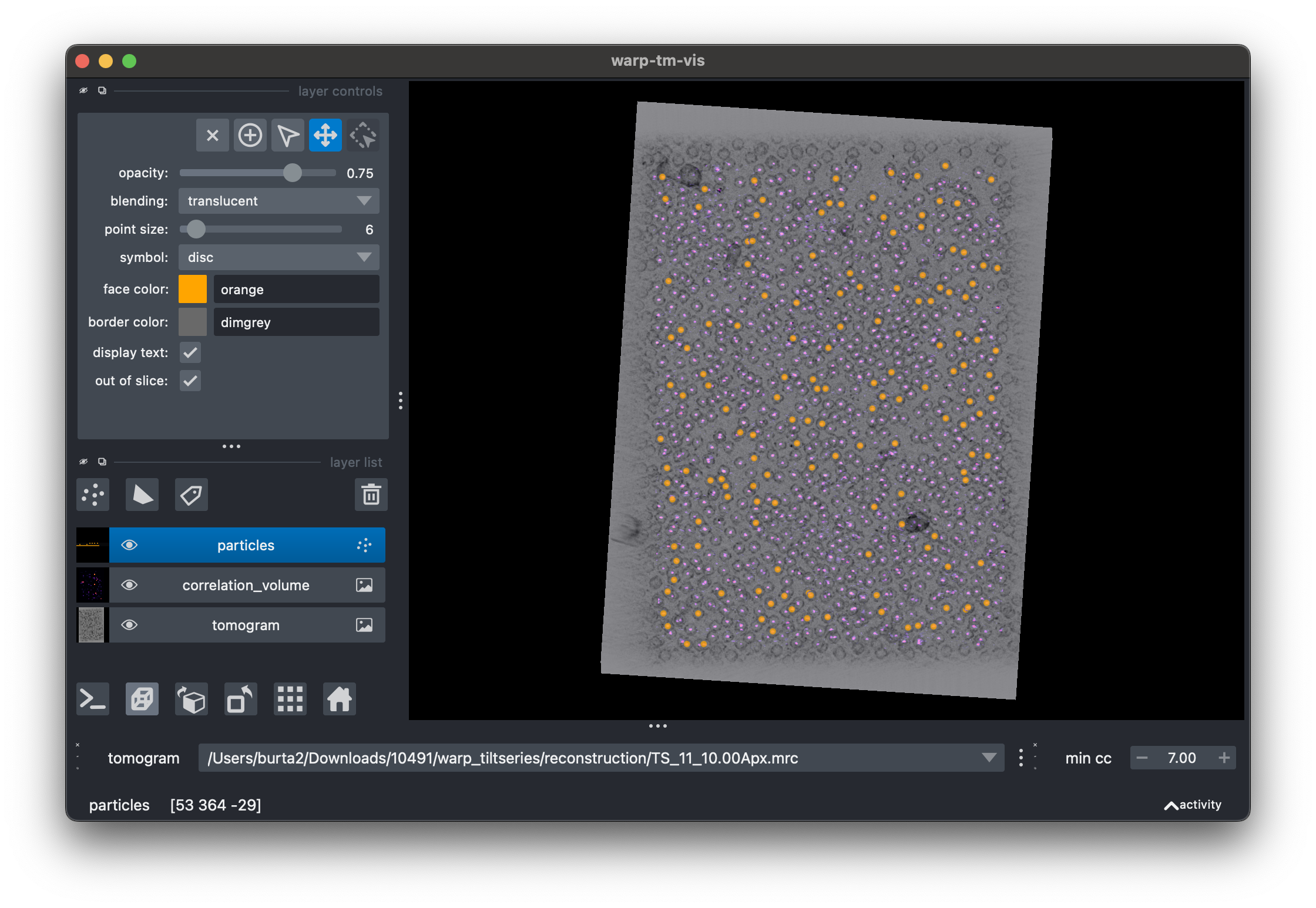
Tip
warp-tm-vis is a graphical application which is designed to be run locally. If your data are on a remote server, download them first before visualizing.
Generating Particle Picks
We can generate particle picks for subsequent processing by finding local maxima in
a thresholded correlation volume. This is done in the threshold_picks WarpTool
WarpTools threshold_picks \
--settings warp_tiltseries.settings \
--in_suffix 15854 \
--out_suffix clean \
--minimum 3
This generates a number of STAR files containing particle positions with a clean
suffix in the filename
warp_tiltseries/matching
├── TS_1_10.00Apx_emd_15854_clean.star
├── TS_11_10.00Apx_emd_15854_clean.star
├── TS_17_10.00Apx_emd_15854_clean.star
├── TS_23_10.00Apx_emd_15854_clean.star
└── TS_32_10.00Apx_emd_15854_clean.star
Export Particles
You can write particles using the ts_export_particles tool as either
- 3D volumes and corresponding CTF volumes
- CTF corrected 2D particle image series
Both output types are compatible with the latest version of RELION, RELION-5. For this tutorial we will write out 2D particle image series. (1)
- if using 3D particles you need to launch refinements from
the
relionGUI, not therelion --tomoGUI.
WarpTools ts_export_particles \
--settings warp_tiltseries.settings \
--input_directory warp_tiltseries/matching \
--input_pattern "*15854_clean.star" \
--normalized_coords \
--output_star relion/matching.star \
--output_angpix 4 \
--box 64 \
--diameter 130 \
--relative_output_paths \
--2d
This will write particle images the warp_tiltseries/particleseries directory.
Per tilt averages (2D or 3D, depending on output dimensionality) are written into
the same directory for debugging, you should see a blob in the center of these images.

Why 4Å per pixel?
The major features of apoferritin are alpha helices which resolve nicely at around 9Å. 9Å is slightly lower than the Nyquist limit of 8Å.
A particle STAR file will be written to the file specified as --output_star. In the
case of 2D averages, a RELION compatible optimisation_set STAR file will be written
out
which points at a description of the tilt series in *_tomograms.star and the
particle star file. This file can be used as input for refinement in the
relion --tomo GUI in RELION 5. A dummy_tiltseries.mrc file is written out for
compatibility with RELION.
relion
├── matching.star
├── matching_tomograms.star
├── matching_optimisation_set.star
└── dummy_tiltseries.mrc
Tip
Want to play with different particle sets at the same time? You can specify
--output_processing to override the processing directory (warp_tiltseries)
in the settings file at any time!
Initial 3D Refinement in RELION
We use RELION to determine good initial particle positions and orientations before attempting high resolution refinements in M. 3D classification in RELION can also be used to separate particles into different classes.
For this apoferritin dataset, an unmasked 3D refinement starting from a 130Å sphere filtered to 60Å refines directly to the Nyquist limit of 8Å.
 Auto-refine: Refinement has converged, stopping now...
 Auto-refine: + Final reconstruction from all particles is saved as: Refine3D/job001/run_class001.mrc
 Auto-refine: + Final model parameters are stored in: Refine3D/job001/run_model.star
 Auto-refine: + Final data parameters are stored in: Refine3D/job001/run_data.star
 Auto-refine: + Final resolution (without masking) is: 8.17021

RELION Refine3D command
This is the command that was run via the RELION --tomo GUI.
mpirun -n 3 `which relion_refine_mpi` \
--o Refine3D/job001/run \
--auto_refine \
--split_random_halves \
--ios matching_optimisation_set.star \
--ref sphere.mrc \
--trust_ref_size \
--ini_high 40 \
--dont_combine_weights_via_disc \
--pool 10 \
--pad 2  \
--ctf \
--particle_diameter 130 \
--flatten_solvent \
--zero_mask \
--oversampling 1 \
--healpix_order 2 \
--auto_local_healpix_order 4\
--offset_range 5 \
--offset_step 2 \
--sym O \
--low_resol_join_halves 40 \
--norm \
--scale  \
--j 2 \
--gpu ""  \
--pipeline_control Refine3D/job001/
High Resolution Refinements in M
While Warp handles the first stages of the data processing pipeline, M lives on its opposite end. It allows you to take refinement results from RELION and perform a multi-particle refinement. For tilt series data, M will likely deliver a noticeable resolution boost compared to initial tilt series alignments from IMOD or AreTomo. Refinement of in situ data will also benefit significantly from the unlimited number of classes and transparent mechanisms for combining data from different sources.
M strives to be a great tool for in situ data, which have been compared to “molecular sociology“. Thus, its terminology takes a somewhat sociological angle. A project in M is referred to as a Population. A population contains at least one Data Source and at least one Species. A Data Source contains a set of frame series or tilt series and their metadata. A Species is a map that is refined, as well as particle metadata for the available data sources.
Setup in MTools
Population Creation
To create a population we run the create_population command from MTools
MTools create_population \
--directory m \
--name 10491
Data Source Setup
Next we create a data source from our tilt series settings file.
MTools create_source \
--name 10491 \
--population m/10491.population \
--processing_settings warp_tiltseries.settings
Species Setup
Create Mask Using RELION
M requires a binary mask around the particle (or region of interest). This mask will be expanded and a soft edge will be added automatically during refinement.
relion_mask_create \
--i relion/Refine3D/job002/run_class001.mrc \
--o m/mask_4apx.mrc \
--ini_threshold 0.04
Setup Species with create_species
Now we create our species, resampling to a smaller pixel size as we hope to reach higher resolution.
MTools create_species \
--population m/10491.population \
--name apoferritin \
--diameter 130 \
--sym O \
--temporal_samples 1 \
--half1 relion/Refine3D/job002/run_half1_class001_unfil.mrc \
--half2 relion/Refine3D/job002/run_half2_class001_unfil.mrc \
--mask m/mask_4apx.mrc \
--particles_relion relion/Refine3D/job002/run_data.star \
--angpix_resample 0.7894 \
--lowpass 10
Running M with MCore
Checking our Setup
First, we run an iteration of M without any refinements to check that everything imported correctly.
MCore \
--population m/10491.population \
--iter 0
This yields a 6.4Å map in our hands.
Tip
--perdevice_refine can be used to run multiple worker processes per GPU
First Refinement
Now we know things have imported correctly we run an iteration of M with 2D image warp
refinement, particle pose refinement and CTF refinement. We use an exhaustive defocus
search
in the first sub-iteration (--ctf_defocusexhaustive) as initial estimates can be quite
far
from the true value and the gradient based optimisation in M may get stuck in local
minima.
MCore \
--population m/10491.population \
--refine_imagewarp 6x4 \
--refine_particles \
--ctf_defocus \
--ctf_defocusexhaustive \
--perdevice_refine 4
This yields a map at 3.6 Å.
Benefits from a Higher Resolution Reference
The reference now has better resolution so we can expect things to improve further without adding any additional parameters.
Tip
Introduce new parameters one by one when refining in M. Be wary of the potential for overfitting parameters if data are weak!
MCore \
--population m/10491.population \
--refine_imagewarp 6x4 \
--refine_particles \
--ctf_defocus
This gave us a modest improvement and we now have a 3.1Å map.
+ Stage Angle Refinement
MCore \
--population m/10491.population \
--refine_imagewarp 6x4 \
--refine_particles \
--refine_stageangles
3.0 A
+ Magnification/Cs/Zernike3
We can add more CTF parameters and see whether this yields any improvements
MCore \
--population m/10491.population \
--refine_imagewarp 6x4 \
--refine_particles \
--refine_mag \
--ctf_cs \
--ctf_defocus \
--ctf_zernike3
In this case, the map stayed at 3.0Å.
+ Weights (Per-Tilt Series)
EstimateWeights \
--population m/10491.population \
--source 10491 \
--resolve_items

MCore \
--population m/10491.population
+ Weights (Per-Tilt, Averaged over all Tilt Series)
EstimateWeights \
--population m/10491.population \
--source 10491 \
--resolve_frames

MCore \
--population m/10491.population \
--perdevice_refine 4 \
--refine_particles
3.0 Å
+ Temporal Pose Resolution
M is capable of refining how particle poses change over time through a tilt series.
MTools resample_trajectories \
--population m/10491.population \
--species m/species/apoferritin_797f75c2/apoferritin.species \
--samples 2

MCore \
--population m/10491.population \
--refine_imagewarp 6x4 \
--refine_particles \
--refine_stageangles \
--refine_mag \
--ctf_cs \
--ctf_defocus \
--ctf_zernike3
2.9 A
Final Map: 2.9Å